CS170 Final Project
🗓 November—December 2019
Project Link: https://github.com/justinvyu/cs170-final-project
Technologies Used
Python, NetworkX
Team 92: ☠️⚰️ NP is no more. (Justin Yu, Dylan Tran, Janice Ng)
Project Summary
Professor Rao and his army of TAs are working in Soda Hall late at night, writing the final exam for CS 170. Rao offers to drive and drop TAs off closer to their homes so that they can all get back safe despite the late hours. However, the roads are long, and Rao would also like to get back to Soda as soon as he can. Can you plan transportation so that everyone can get home as efficiently as possible?
Formally, you are given an undirected graph \(G = (L,E)\) where each vertex in \(L\) is a location. You are also given a starting location s, and a list H of unique locations that correspond to homes. The weight of each edge \((u, v)\) is the length of the road between locations u and v, and each home in H denotes a location that is inhabited by a TA. Traveling along a road takes energy, and the amount of energy expended is proportional to the length of the road. For every unit of distance traveled, the driver of the car expends 2/3 units of energy, and a walking TA expends 1 unit of energy.
The car must start and end at \(s\), and every TA must return to their home in \(H\). You must return a list of vertices that is the tour taken by the car (cycle with repetitions allowed), as well as a list of drop-off locations at which the TAs get off. You may only drop TAs off at vertices visited by the car, and multiple TAs can be dropped off at the same location.
We’d like you to produce a route and sequence of drop-offs that minimizes total energy expenditure, which is the sum of Rao’s energy spent driving and the total energy that all of the TAs spend walking. Note TAs do not expend any energy while sitting in the car. You may assume that the TAs will take the shortest path home from whichever location they are dropped off at.
Inputs
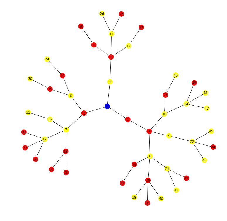
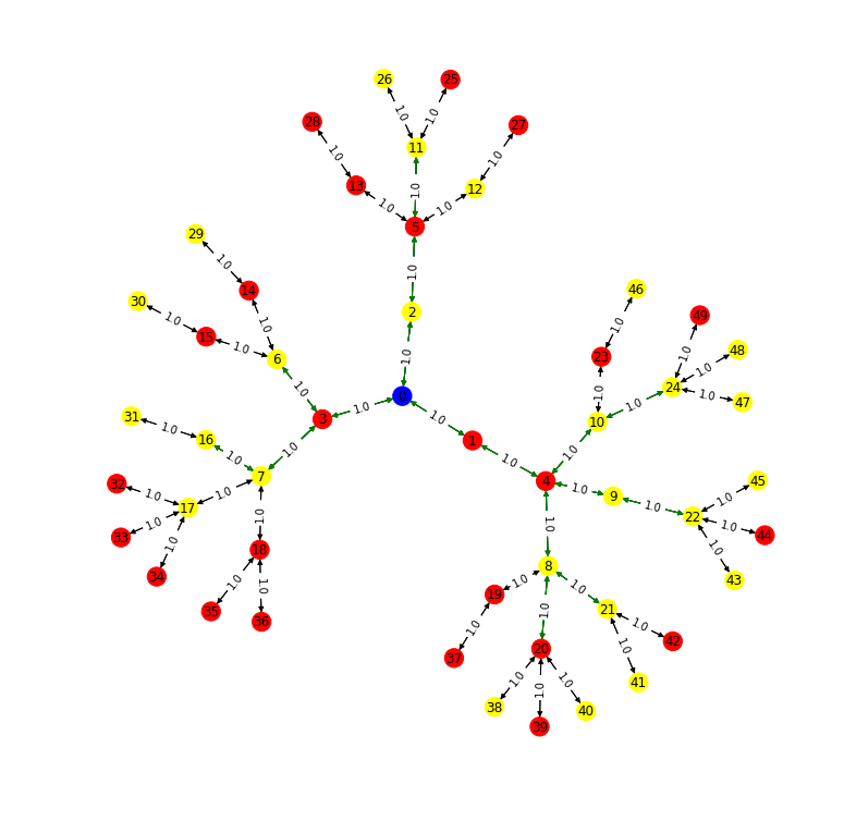
50 Houses Input
25 TAs, whose houses are in yellow. The blue vertex is the source/starting location.
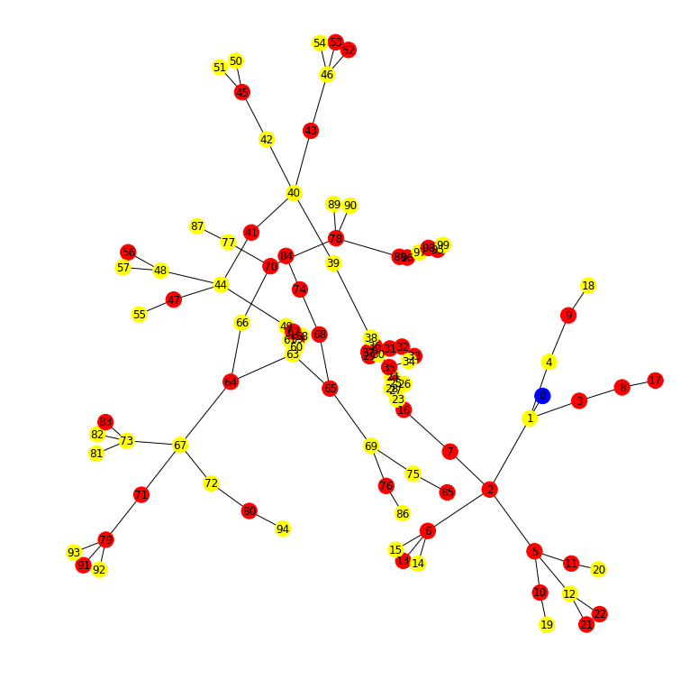
100 Houses Input
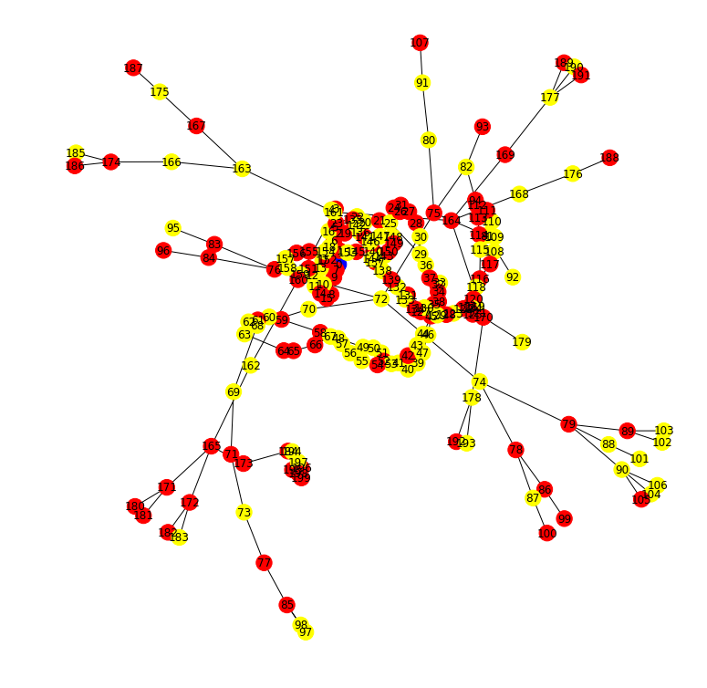
200 Houses Input
Solver Summaries
MST+DFS: We used the MST + DFS approximation for MetricTSP as a baseline for other solutions to improve upon. However, since the original graph is not necessarily fully connected, not every duplicate vertex seen can be removed. This solution drops everyone off at their houses, with no walking TAs. This may be inefficient, because when there are multiple branching paths, the car expends (4/3) more energy than a solution that drops off the TAs at the intersection.
Greedy: Our second approach was a greedy solver that decided which neighbor to travel to at each step in the iteration. Once all TAs have been dropped off, it takes the shortest path back to the source. We employed a heuristic to determine which of the neighbors is the best direction to move. At any given vertex u, with neighbors v, the heuristic was \(heurstic(v) = \sum_{h}^{} (\frac{1}{dist(v, h)})^2\), where \(dist(v, h)\) is the shortest distance from neighbor v to the house h. This solver didn’t perform better than the naive MST+DFS solver on many inputs, because the metric sometimes took inefficient routes or doubled back on certain locations where the heuristic wasn’t perfect in determining the best neighbor.
To improve upon the above, we created solvers for two different approaches:
Approach (1): Find dropoff points, then assign a closed walk that goes through all of them. Drop people off based on the location they are closest to.
FLP: The first solver falling under approach (1) was based on the Facility Location Problem (FLP). We used an FLP to set cover reduction and used a greedy set cover solver to approximate FLP and extended FLP to estimate DTH. The FLP is a problem that involves choosing locations to place facilities to service a set of all clients. We formulated the following problem:
- D clients = D homes
- Set F of potential facilities = all locations (potential dropoffs locations)
- Distance function = shortest path between a pair of vertices (Floyd Warshall)
- Cost function for facility = ⅔ * distance from start to dropoff
- We minimize the sum of placing all dropoffs + the sum of the distances to the homes of the TAs we drop there
Intuitively, doing FLP allows us to cluster homes centered around a potential dropoff location and choose the best among potential locations and select facility sites to minimize costs (https://www.cs.cmu.edu/~anupamg/adv-approx/lecture4.pdf). We modify this algorithm in two ways:
- Updating the cost of placing facilities to be distance from nearest dropoff in the set of chosen dropoffs in each iteration
- If (i, A) is chosen to be included, we remove the cost of placing a facility (distance from start) for all i’s in set S
Once we identify dropoffs, we greedily find a path from start through all of them and back. Then, assign homes to the nearest dropoff.
K-means Clustering: The second solver falling under (1) is a solver that first finds k dropoff locations through k-means clustering. For each graph, we searched over the number of clusters k from 1 to |H|, the number of houses, and picked the k with the minimum cost. Then, we assigned a path through all of these k dropoff locations and back to the source (by using the MST+DFS solver on a partial MST containing only points needed to reach the k centers), and we assigned drop-offs for each house to the nearest cluster center. We found that this solution does well, but doesn’t do any better than the local search solver.
Approach (2): Find a closed walk and assign optimal dropoff locations given this tour of the graph, then make changes to the closed walk to optimize.
Local Search: The local search solver iteratively optimizes an initial closed walk that is passed in. To do this, we first define a neighborhood to include closed walks that: (a) include exactly one more vertex or (b) exclude exactly one vertex. This gives a bound of \(O(# vertices)\) neighbors at each iteration. We define the neighborhood conservatively to preserve a polynomial runtime. At each iteration in the solver, we assign dropoffs optimally (to the closest location on the path) and evaluate the cost. We replace the current solution with the neighbor with the minimum cost. If all neighbors have higher cost, then terminate. This is the idea of hill climbing, which might end up in a local optimum.
Which algorithm performed the best?
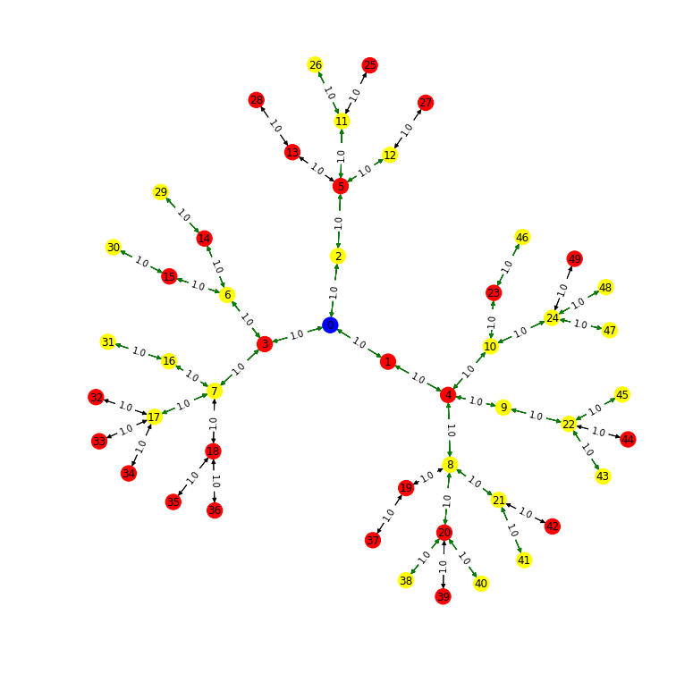
In the traversals below, the green edges are part of the car’s path, and black edges are not part of the path.

MST + DFS
The driving cost of your solution is 65.33333333333333. The walking cost of your solution is 0. The total cost of your solution is 65.33333333333333.
Greedy
The driving cost of your solution is 46.666666666666664. The walking cost of your solution is 0. The total cost of your solution is 46.666666666666664.

K-means Cluster + Local Search
BEST SOLUTION WITH 1 CLUSTERS, COST=46.666666666666664. The driving cost of your solution is 24.0. The walking cost of your solution is 17.0. The total cost of your solution is 41.0.
FLP + Local Search
The driving cost of your solution is 22.666666666666668. The walking cost of your solution is 17.0. The total cost of your solution is 39.66666666666667.
We used the local search algorithm as a post-processing step, so all of the other solvers’ solutions were passed into iterations of local search to optimize the solution further. Since the local search algorithm only swaps with a neighbor if the cost is smaller, it will never make a solution worse than it was originally. Starting from the naive MST+DFS solution, local search optimizations give a solution that are similar in quality as the FLP outputs. However, passing the FLP solution into local search improved the cost even more. The MST-DFS solver usually performed the worst as it dropped all the TAs off instead of searching for walking paths to reduce energy, which is why we think the local search/FLP solutions did better.
Future Improvements
First, we would increase the number of neighbors considered in the local search to prevent getting stuck at a local optimum. Since the hill climbing algorithm stops once all neighbors have higher cost, the conservative neighborhood means that there may be a close solution out there that we do not consider that has lower cost, but we terminate early because the “neighborhood” is not big enough. Second, we would implement and tune an exploration strategy such as simulated annealing to make it less likely to converge to a local optimum. Third, in the solvers falling under approach (1), we greedily finding paths through drop offs by considering the shortest path each time. Here, we could have used a better TSP approximation such as using an ILP solver or Christofides’ algorithm.